Monkeys love to make a mess. Monkeys like to throw stones. Give a monkey a bucket of small pebbles, and before too long, those pebbles will be scattered indiscriminately in all directions. These are true facts about monkeys, facts we can exploit for the construction of a random number generator.
Set up a room full of empty buckets. Add one bucket full of pebbles and one mischievous monkey. Once the pebbles have been scattered, the number of little stones in each bucket is a random variable. We're going to use this random number generator for an unusual purpose, though. In fact, we could call it a 'calculus of probability,' because we're going to use this exotic apparatus for figuring out probability distributions from first principles1.
Lets say we have a hypothesis space consisting of n mutually exclusive and exhaustive propositions. We need to find a prior probability distribution over this set of hypotheses, so we can begin the process of Bayesian updating, using observed data. But nobody can tell us what the prior distribution ought to be, all we have is a limited set of structural constraints - we know the whole distribution must sum to 1, and perhaps we can deduce other properties, such as an appropriate mean or standard deviation. So we design an unusual experiment to help us out. We need to lay out n empty buckets - one bucket for each hypothesis in the entire set of possibilities (better nail them to the floor).
Each little pebble that we give to the monkey represents a small unit of probability, so the arrangement of stones in buckets at the end represents a candidate probability distribution. We've been very clever, beforehand, and we've made sure that the resting place of each pebble is uniformly randomly distributed over the set of buckets - in keeping with everything we've heard about the chaotic nature of monkeys, this one exhibits no systematic bias - so we decide that this candidate probability distribution is a fair sample from among all the possibilities.
We examine the candidate distribution, and check that it doesn't violate any of our known constraints. If it does violate any constraints, then it's no use to us, and we have to forget about it. If not, we record the distribution, then go tidy everything up, so we can repeat the whole process again. And again. And again and again and again, and again. After enough cycles, there should be a clear winner, one distribution that occurs more often than any other. This will be the probability distribution that best approximates our state of knowledge.
To convince ourselves that some distributions really will occur significantly more frequently than others, we just need to do a little combinatorics. Suppose the total supply of ammo given to the little beast comes to N pebbles.
The number of possible ways to end up with exactly N1 pebbles in the first bucket is given by the binomial coefficient:

and with those N1 pebbles accounted for, the number of ways to get exactly N2 in the second bucket is

and so on.
So the total number of opportunities to get some particular distribution of stones (probability mass) over all n buckets (hypotheses) is given by the product
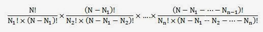
For each ith term in this product (up to n-1), the term in brackets in the denominator is the same as the numerator of the (i+1)th term, so these all cancel out, and for the nth term, the corresponding part of the denominator comes to 0!, which is 1. So any particular outcome of this experiment can, in a long run of similar trials, be expected to occur with frequency proportional to

which we call the multiplicity of the particular distribution defined by the numbers N1, N2, ...., Nn.
The number of buckets, n, only needs to be moderately large for it to be quite difficult to visualize how W varies as a function of the Ni. We can get around this by looking into the case of only 2 buckets. Below, I've plotted the multiplicity as a function of the fraction of stones in the first of two available buckets, for three different total numbers of stones: 50, 500, and 1000 (blue and green curves enhanced to come up to the same height as the red curve).

Each case is characterized by a fairly sharp peak, centered at 50%. As the number of stones available increases, so does the sharpness of the peak - it becomes less and less plausible for the original supply of pebbles to end up very unequally divided between the available resting places.
Calculating large factorials is quite tricky work, though (just look at the numbers: 2.7 × 10299, for N = 1000). To find which distribution is expected to occur most frequently, we need to locate the arrangement for which W is maximized, but any monotonically increasing function of W will be maximized by the same distribution, so instead lets maximize another function, which I'll arbitrarily call H:

But since each Ni is N×pi (where pi is the probability for any given stone to land in the ith bucket, according to this distribution), and repeatedly using the quotient rule for logs,

Now, because probabilities vary over a continuous range between 0 and 1, and because we don't wan't to impose overly artificial constraints on the outcome of the experiment, we will have given the monkey a really, really large number of pebbles. This means that we can simplify the above expression for H using the Stirling approximation, which states generally that when k is very large (where we're using the natural base),

with the approximation getting better as k gets larger. In our particular case, this yields

and suddenly, we can see why that 1/N was inexplicably sitting at the front of our expression for H:

The Σpi term at the end is 1, so

at which point the product rule for logs produces
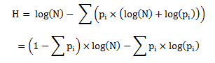
finally, yielding

which, oh my goodness gracious, is exactly the same as the quantity we had previously labelled H: the Shannon entropy.
So, it turns out that the probability distribution most likely to come out favorite in the repeated monkey experiment, the one corresponding to the arrangement of stones with the highest multiplicity, and therefore the one best expressing our state of ignorance, is the one with the highest entropy. And this is the maximum entropy principle. It means that any distribution with lower entropy than is permitted by the constraints present in the problem has somehow incorporated more information that is actually available to us, and so adoption of any such distribution constitutes an irrational inference.
Note, though, that if your gut feeling is that the maximum entropy distribution you've calculated is not specific enough, this is your gut expressing the opinion that you actually do have some prior information that you've neglected to include. It's probably worth exploring the possibility that your gut is right.
It might seem, from this multiplicity argument, that for a given number of points, n, in the hypothesis space, there is only one possible maximum entropy distribution, but recall that sometimes (as in the kangaroo problem) we have information from which we can formulate additional constraints. Sometimes the unconstrained maximum-multiplicity distribution will be ruled out by these constraints, and we have to select a distribution from those that aren't ruled out. It's in such cases that the method actually gets interesting and useful.
This hasn't been Jaynes' original derivation of the maximum entropy principle (the logic presented here was brought to Jaynes' attention by G. Wallis), and neither is it a rigorous mathematical proof, but it has the substantial advantage of intuitive appeal. It even makes concrete the abstract link between the maximum entropy principle and the second law of thermodynamics.
Thinking again about the expanding gas example from the previous post, we can see the remarkable similarity between the simple universe we considered then, a box containing 100 gas molecules, with the space inside the box conceptually divided into 32 equal-sized regions, and the apparatus described here. The expanding gas scenario corresponds very closely to a possible instance of the monkey experiment with 32 buckets and 100 pebbles:

As the multiplicity curves above testify, the state with the highest multiplicity is the one with as close as possible to equal numbers of molecules in each region, so a state like the one above is far more likely than one in which one half of the box is empty. Given the fact that the gas molecules move about, in a highly uncorrelated way, therefore, we can see that the second law of thermodynamics (the fact that a closed system in a low-entropy state now will tend to move to and stay in a high-entropy state) amounts to a tautology: if there is a more probable state available, then expect to find the system in that state next time you look.
We also saw above that increasing the number of pebbles / molecules reduces the relative width of the multiplicity curve. But the numbers of particles encountered in typical physical situations are astronomically huge. In a cubic meter of air, for example, at sea level and around room temperature, there are (from the ideal-gas approximation) around 2.5 × 1025 molecules (which, by the way, weighs roughly 1 kg). This means that once a system like this gas-in-a-box experiment has evolved to its state of highest entropy, the chances of seeing the entropy decrease again by any appreciable amount vanish completely. Thus the second tendency of thermodynamics receives a well earned promotion, and we call it instead 'the second law'.
Please note: no primates were harmed during the making of this post.
References
Now, because probabilities vary over a continuous range between 0 and 1, and because we don't wan't to impose overly artificial constraints on the outcome of the experiment, we will have given the monkey a really, really large number of pebbles. This means that we can simplify the above expression for H using the Stirling approximation, which states generally that when k is very large (where we're using the natural base),
with the approximation getting better as k gets larger. In our particular case, this yields
and suddenly, we can see why that 1/N was inexplicably sitting at the front of our expression for H:
The Σpi term at the end is 1, so
at which point the product rule for logs produces
finally, yielding
which, oh my goodness gracious, is exactly the same as the quantity we had previously labelled H: the Shannon entropy.
So, it turns out that the probability distribution most likely to come out favorite in the repeated monkey experiment, the one corresponding to the arrangement of stones with the highest multiplicity, and therefore the one best expressing our state of ignorance, is the one with the highest entropy. And this is the maximum entropy principle. It means that any distribution with lower entropy than is permitted by the constraints present in the problem has somehow incorporated more information that is actually available to us, and so adoption of any such distribution constitutes an irrational inference.
Note, though, that if your gut feeling is that the maximum entropy distribution you've calculated is not specific enough, this is your gut expressing the opinion that you actually do have some prior information that you've neglected to include. It's probably worth exploring the possibility that your gut is right.
It might seem, from this multiplicity argument, that for a given number of points, n, in the hypothesis space, there is only one possible maximum entropy distribution, but recall that sometimes (as in the kangaroo problem) we have information from which we can formulate additional constraints. Sometimes the unconstrained maximum-multiplicity distribution will be ruled out by these constraints, and we have to select a distribution from those that aren't ruled out. It's in such cases that the method actually gets interesting and useful.
This hasn't been Jaynes' original derivation of the maximum entropy principle (the logic presented here was brought to Jaynes' attention by G. Wallis), and neither is it a rigorous mathematical proof, but it has the substantial advantage of intuitive appeal. It even makes concrete the abstract link between the maximum entropy principle and the second law of thermodynamics.
Thinking again about the expanding gas example from the previous post, we can see the remarkable similarity between the simple universe we considered then, a box containing 100 gas molecules, with the space inside the box conceptually divided into 32 equal-sized regions, and the apparatus described here. The expanding gas scenario corresponds very closely to a possible instance of the monkey experiment with 32 buckets and 100 pebbles:
As the multiplicity curves above testify, the state with the highest multiplicity is the one with as close as possible to equal numbers of molecules in each region, so a state like the one above is far more likely than one in which one half of the box is empty. Given the fact that the gas molecules move about, in a highly uncorrelated way, therefore, we can see that the second law of thermodynamics (the fact that a closed system in a low-entropy state now will tend to move to and stay in a high-entropy state) amounts to a tautology: if there is a more probable state available, then expect to find the system in that state next time you look.
We also saw above that increasing the number of pebbles / molecules reduces the relative width of the multiplicity curve. But the numbers of particles encountered in typical physical situations are astronomically huge. In a cubic meter of air, for example, at sea level and around room temperature, there are (from the ideal-gas approximation) around 2.5 × 1025 molecules (which, by the way, weighs roughly 1 kg). This means that once a system like this gas-in-a-box experiment has evolved to its state of highest entropy, the chances of seeing the entropy decrease again by any appreciable amount vanish completely. Thus the second tendency of thermodynamics receives a well earned promotion, and we call it instead 'the second law'.
Please note: no primates were harmed during the making of this post.
References
| [1] |
I can't claim credit for designing this monkey experiment. Versions of it are dotted about the literature, possibly originating with:
Gull, S.F. and Daniell, G.J., Image Reconstruction from Incomplete and Noisy Data, Nature 272, no. 20, page 686, 1978
See also
Jaynes, E.T., Monkeys, Kangaroos, and N, in Maximum-Entropy and Bayesian Methods in Applied Statistics, edited by Justice, J.H., Cambridge University Press, 1986 (full text of the paper available here)
|
Hi Tom,
ReplyDeleteSuppose we give our monkey an infinite amount of stones and lay out an infinite amount of buckets - what happens then?
We also have an infinite supply of monkeys ;)
A very good question.
DeleteAlthough also a bad question! It's a bad question, because it is ill-posed - there's no number called infinity anywhere on the number line, as I'm sure you appreciate. So in order to do calculations with infinity, we have to specify some means to get there as a limit, of which there are many possibilities, giving many different results (many of which will be nonsensical).
Its a good question, because if we choose a suitable limiting process that maintains the relationship N >> n, then we'll find out that the maximum entropy principle, applied to the discrete entropy function I've been using, also covers an analogous function for continuous hypothesis spaces, which is rather useful.
See here for a brief discussion of the continuous entropy function.